# Install and load the necessary package
library(plm)63 Advanced Time-Series Models - Panel Data Practical
63.1 Introduction
In this section, I’m going to introduce another approach - panel data - to analysing data collected over time that is commonly found in sport data analytics (e.g., Sabermetrics).
Panel data, also known as ‘longitudinal data’ or ‘cross-sectional time-series data’, consists of observations of multiple phenomena over multiple time periods. In the context of time-series analysis, panel data allows us to analyse dynamics across both entities (like individuals, teams, leagues, etc.) and time.
So, panel data is used to analyse data collected from the same entity repeatedly over a period of time. It’s particularly valuable because it allows us to observe differences:
- between different athletes/teams/groups and
- over time.
63.2 Panel Data - demonstration
First, I’ll load the plm package which is used for panel data.
Now, I’ll create a simple dataset for 6 teams, collected over 4 seasons.
The dataset contains the total goals scored, the total assists, and the total fouls.
library(ggplot2)

set.seed(123)

teams <- paste("Team", 1:6)
seasons <- 1:4

# Create data frame
num_teams <- length(teams)
num_seasons <- length(seasons)
observations <- num_teams * num_seasons

team_data <- expand.grid(team = teams, season = seasons)
team_data$goals <- rpois(observations, lambda = 30)
team_data$assists <- rpois(observations, lambda = 20)
team_data$fouls <- rpois(observations, lambda = 10)

# View dataset
head(team_data)
team season goals assists fouls
1 Team 1 1 26 18 5
2 Team 2 1 36 14 6
3 Team 3 1 20 24 10
4 Team 4 1 30 23 11
5 Team 5 1 39 23 8
6 Team 6 1 32 23 8There are four steps to panel data analysis.
First, I convert the data into a pdata frame. Note that this creates a new dataframe with time and group identifiers as the row (observation) names.
# Convert the data frame to a pdata.frame for panel analysis
panel_data <- pdata.frame(team_data, index = c("team", "season"))
Second, I conduct some exploratory analysis on the data.
# EDA: Plotting goals over seasons by team
ggplot(panel_data, aes(x = season, y = goals, group = team, color = team)) +
  geom_line() +
  geom_point() +
  theme_minimal() +
  labs(title = "Total Goals Over 4 Seasons, by Team", x = "Season", y = "Goals")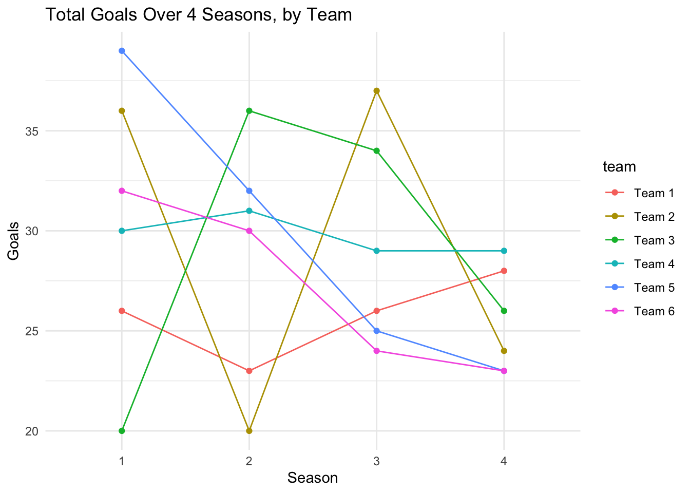
Third, I create a fixed-effects model.
In this model, I’m trying to understand the impact of within-team variations over time.
By using a fixed effects model, we try to identify whether changes in the number of assists and fouls within the same team across different seasons have a significant effect on the goals they score, controlling for the unobserved, time-invariant characteristics unique to each team.
Note: a fixed-effects model doesn’t take account of the fact that you have group-level differences. It ignores any impact of ‘difference’. MLM.
# Fit a fixed effects model
fe_model <- plm(goals ~ assists + fouls, data = panel_data, model = "within")
summary(fe_model)
Oneway (individual) effect Within Model
Call:
plm(formula = goals ~ assists + fouls, data = panel_data, model = "within")
Balanced Panel: n = 6, T = 4, N = 24
Residuals:
Min. 1st Qu. Median 3rd Qu. Max.
-8.913569 -3.675609 0.025616 3.433283 9.128307
Coefficients:
Estimate Std. Error t-value Pr(>|t|)
assists 0.015223 0.370213 0.0411 0.9677
fouls -0.650180 0.711328 -0.9140 0.3743
Total Sum of Squares: 615.75
Residual Sum of Squares: 585.11
R-Squared: 0.049768
Adj. R-Squared: -0.36596
F-statistic: 0.419 on 2 and 16 DF, p-value: 0.66472library(broom)
# Visualise the coefficients from the fixed effects model
coef_df <- tidy(fe_model)
ggplot(coef_df, aes(x = term, y = estimate)) +
geom_point() +
geom_errorbar(aes(ymin = estimate - std.error, ymax = estimate + std.error), width = 0.2) +
labs(title = "Fixed Effects Model Coefficients", x = "Predictors", y = "Estimates")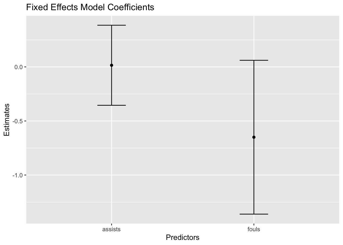
Finally, I create a random-effects model.
Using this type of model extends my analysis to examine whether the observed relationships between assists, fouls, and goals are generalisable across different teams. A random effects model is used to assess whether the impacts of assists and fouls on goals are consistent not just within teams over time but also across different teams, accounting for both within-team and between-team variations.
# Fit a random effects model
re_model <- plm(goals ~ assists + fouls, data = panel_data, model = "random")
summary(re_model)
Oneway (individual) effect Random Effect Model
(Swamy-Arora's transformation)
Call:
plm(formula = goals ~ assists + fouls, data = panel_data, model = "random")
Balanced Panel: n = 6, T = 4, N = 24
Effects:
var std.dev share
idiosyncratic 36.569 6.047 1
individual 0.000 0.000 0
theta: 0
Residuals:
Min. 1st Qu. Median 3rd Qu. Max.
-8.3322 -4.5250 -0.1928 3.5236 10.6038
Coefficients:
Estimate Std. Error z-value Pr(>|z|)
(Intercept) 30.484327 8.061795 3.7813 0.000156 ***
assists -0.056959 0.325748 -0.1749 0.861192
fouls -0.097260 0.549590 -0.1770 0.859533
---
Signif. codes: 0 '***' 0.001 '**' 0.01 '*' 0.05 '.' 0.1 ' ' 1
Total Sum of Squares: 667.96
Residual Sum of Squares: 665.87
R-Squared: 0.0031195
Adj. R-Squared: -0.091822
Chisq: 0.0657136 on 2 DF, p-value: 0.96768# Visualise coefficients from random effects model
re_coef_df <- tidy(re_model)
ggplot(re_coef_df, aes(x = term, y = estimate)) +
geom_point() +
geom_errorbar(aes(ymin = estimate - std.error, ymax = estimate + std.error), width = 0.2) +
labs(title = "Random Effects Model Coefficients", x = "Predictors", y = "Estimates")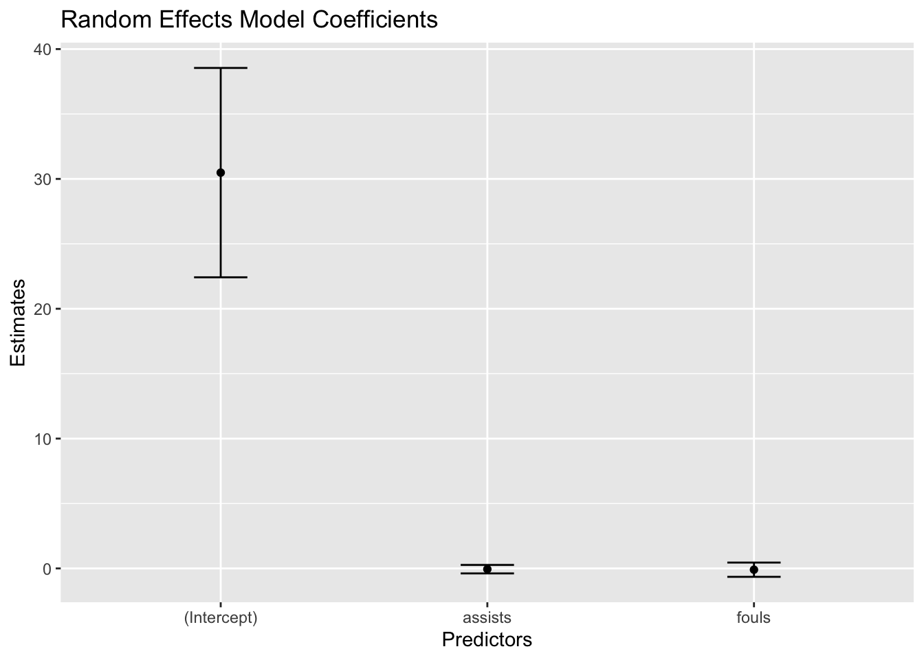
This is a plot of the estimated coefficients from the random effects model, along with their corresponding confidence intervals.
It gives us a visual representation of the impact each predictor (assists and fouls) has on the dependent variable (goals) in the model.
By comparing the coefficient plots of the fixed and random effects models, we can examine how assumptions about individual variability influence the estimation of effects in panel data analysis.
Note that, in the context of most panel data analyses in sport, the intercept might not hold a practical interpretation as our values are rarely zero.
63.3 Further examples
63.3.1 Step one: preparation
I’ll create another synthetic dataset.
In this case, we’re interested in analysing each player’s performance across different seasons, and also how each player’s performance compares with the others.
The dataset includes player ID, season, goals scored, assists, and minutes played.
rm(list=ls())
# load packages
library(plm)

# Creating synthetic data
set.seed(123) # for reproducibility
players <- data.frame(
  player_id = rep(1:10, each=5),
  season = rep(2010:2014, times=10),
  goals = sample(0:30, 50, replace = TRUE),
  assists = sample(0:20, 50, replace = TRUE),
  minutes_played = sample(1800:3600, 50, replace = TRUE)
)
63.3.2 Step two: explore the data
Now, we’ll explore our data.
# Basic exploration
head(players)
player_id season goals assists minutes_played
1 1 2010 30 6 2409
2 1 2011 14 20 2129
3 1 2012 18 5 2525
4 1 2013 13 1 1926
5 1 2014 2 4 2011
6 2 2010 9 7 2485summary(players) player_id season goals assists minutes_played
Min. : 1.0 Min. :2010 Min. : 2.00 Min. : 0.00 Min. :1838
1st Qu.: 3.0 1st Qu.:2011 1st Qu.: 8.25 1st Qu.: 5.25 1st Qu.:2232
Median : 5.5 Median :2012 Median :14.00 Median :11.00 Median :2617
Mean : 5.5 Mean :2012 Mean :15.38 Mean :10.40 Mean :2667
3rd Qu.: 8.0 3rd Qu.:2013 3rd Qu.:23.50 3rd Qu.:15.00 3rd Qu.:3108
Max. :10.0 Max. :2014 Max. :30.00 Max. :20.00 Max. :3592 We can visualise some of the trends within the data. For example:
library(ggplot2)
library(dplyr)
Attaching package: 'dplyr'The following objects are masked from 'package:plm':
between, lag, leadThe following objects are masked from 'package:stats':
filter, lagThe following objects are masked from 'package:base':
intersect, setdiff, setequal, unionggplot(players, aes(x = season, y = goals, group = player_id, color = as.factor(player_id))) +
geom_line() +
geom_point() +
theme_minimal() +
labs(title = "Trend of Goals Scored Over Four Seasons, by Player",
x = "Season",
y = "Goals",
color = "Player ID")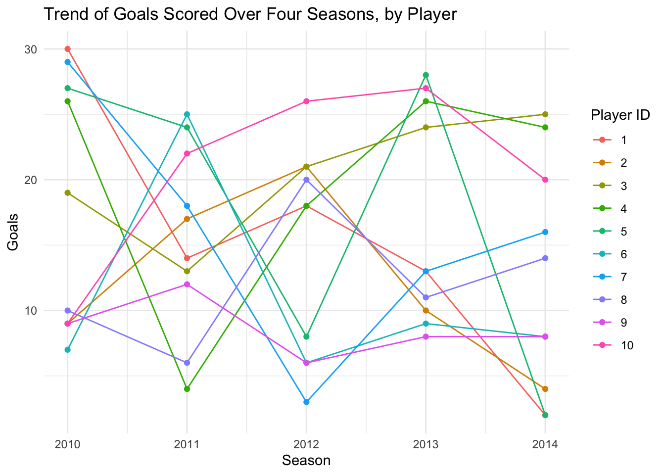
players %>%
  group_by(season) %>%
  summarize(average_assists = mean(assists)) %>%
  ggplot(aes(x = season, y = average_assists)) +
  geom_line() +
  geom_point() +
  theme_minimal() +
  labs(title = "Average Assists Per Season",
       x = "Season",
       y = "Average Assists")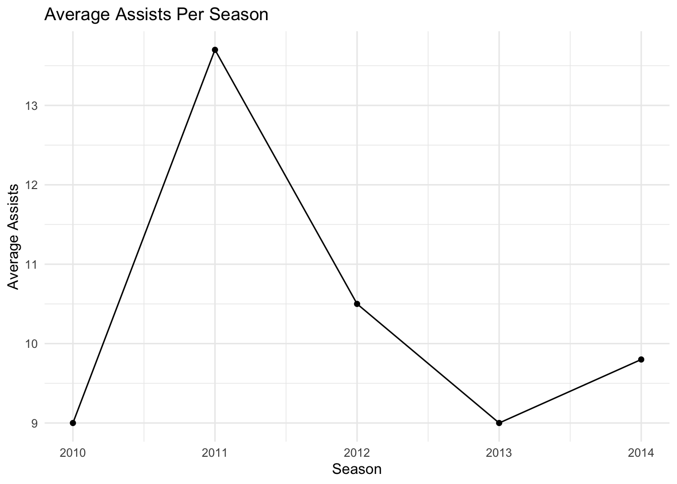
ggplot(players, aes(x = minutes_played, y = goals)) +
  geom_point() +
  geom_smooth(method = "lm", color = "blue") +
  theme_minimal() +
  labs(title = "Relationship Between Goals and Minutes Played",
       x = "Minutes Played",
       y = "Goals")
`geom_smooth()` using formula = 'y ~ x'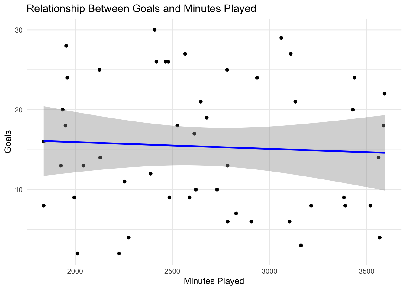
63.3.3 Step three: fit the panel model
Now, we’re going to fit a panel model.
Let’s say we’ve made our research question more specific. We want to understand how the number of goals scored by a player is influenced by the number of minutes they played and the number of assists they made, considering both individual player effects and time effects.
Remember, in panel models we can use either a fixed-effects model or a random-effects model.
Fixed-effects models are great for looking at how specific changes or actions affect the same team or player over time.
- For example, if you want to study how a new training program impacts a basketball team’s performance, a fixed-effects model would allow you to see the effects of this program by comparing the team’s performance before and after its implementation, focusing on the changes within this specific team.
On the other hand, random-effects models are useful when you want to compare general trends across different teams or players, especially when these teams or players are not related to the things you are measuring.
- For instance, if you’re examining how age affects the performance of football players across various teams, a random-effects model would help you understand this broader relationship without getting too caught up in the unique characteristics of each player or team.
63.3.3.1 A fixed-effects model
Fixed-effects models assume that the individual effects (e.g., player or team-specific effects) are correlated with the independent variables. They assume that these unique attributes can have their own impact on the dependent variable.
Fixed-effects models analyse the impact of variables that vary over time. They control for all time-invariant characteristics of the individuals, thereby removing the effect of those time-invariant characteristics from the predictors.
We’d use a fixed-effects model when wewant to examine the causal relationships or effects of time-varying predictors within an entity (e.g., how a player’s performance changes over time due to specific training programs).
Fixed-effects model essentially use within-entity variations for estimation, ignoring between-entity variations.
Let’s build a fixed-effects model using the player data.
# Fit a fixed effects model
fe_model <- plm(goals ~ minutes_played + assists, data=players,
                model="within", index=c("player_id", "season"))
summary(fe_model)
Oneway (individual) effect Within Model
Call:
plm(formula = goals ~ minutes_played + assists, data = players,
model = "within", index = c("player_id", "season"))
Balanced Panel: n = 10, T = 5, N = 50
Residuals:
Min. 1st Qu. Median 3rd Qu. Max.
-15.62521 -3.24657 -0.55551 4.88182 14.52497
Coefficients:
Estimate Std. Error t-value Pr(>|t|)
minutes_played -0.00026217 0.00241461 -0.1086 0.9141
assists -0.10818727 0.21319487 -0.5075 0.6148
Total Sum of Squares: 2536.8
Residual Sum of Squares: 2519.7
R-Squared: 0.0067362
Adj. R-Squared: -0.28079
F-statistic: 0.128855 on 2 and 38 DF, p-value: 0.87948In this model, we’re trying to understand how the independent variables (minutes_played and assists) are associated with the dependent variable (goals) while controlling for individual-specific characteristics that are constant over time (i.e., player-specific effects).
In the output above, we can see a number of elements of information:
Coefficients (Estimate): These represent the estimated impact of each independent variable on the dependent variable. For instance, if the coefficient of
minutes_playedis 0.01, it suggests that for each additional minute played, a player is expected to score 0.01 more goals, holding other factors constant.Standard Errors: These indicate the precision of the coefficient estimates. Smaller standard errors suggest greater precision.
T-values and P-values: These are used for hypothesis testing. The t-value tests the null hypothesis that the coefficient is zero (no effect). The p-value tells you the probability of observing such a t-value if the null hypothesis were true. Typically, a p-value less than 0.05 is considered statistically significant, meaning there’s less than a 5% chance that the observed association is due to random chance.
R-squared and Within R-squared: R-squared values measure the proportion of variance in the dependent variable that’s explained by the independent variables. In fixed-effects models, the ‘Within R-squared’ is more relevant as it considers variation over time within each panel unit (player).
F-statistic: This tests whether the model as a whole has explanatory power, i.e., whether all the coefficients in the model are jointly different from zero.
Interpretation: The output of our fixed-effects model shows:
A coefficient of >0 for minutes_played with a p-value of 0.91. A coefficient of -0.11 for assists with a p-value of 0.6. A within R-squared of 0.07. You would interpret this as:
So there are no
Imagine that the results had been:
A coefficient of 0.02 for
minutes_playedwith a p-value of 0.03.A coefficient of 0.5 for
assistswith a p-value of 0.01.A within R-squared of 0.70.
You would interpret this as:
For each additional minute played, a player is expected to score 0.02 more goals, and this effect is statistically significant (p < 0.05).
Each additional assist is associated with an increase of 0.5 goals scored by a player, and this association is statistically significant (p < 0.05).
70% of the variation in goals scored within players over time is explained by the number of minutes played and assists.
Here are some visualisations of the model:
library(plm)
library(ggplot2)
library(broom)

# Coefficient plot

coef_df <- tidy(fe_model)
ggplot(coef_df, aes(x = term, y = estimate)) +
geom_point() +
geom_errorbar(aes(ymin = estimate - std.error, ymax = estimate + std.error), width = 0.2) +
xlab("Variables") +
ylab("Estimates") +
ggtitle("Coefficient Plot for Fixed Effects Model")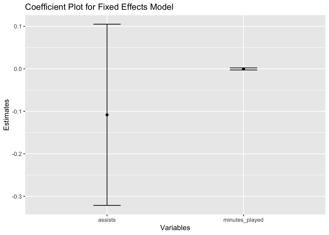
# Time-Series Plot for specific player

player_data <- pdata.frame(players, index = c("player_id", "season"))
player_specific <- player_data[player_data$player_id == "2", ]
player_specific$fitted_values <- predict(fe_model, newdata = player_specific)

ggplot(player_specific, aes(x = season)) +
  geom_point(aes(y = fitted_values), color = "blue") +
  geom_point(aes(y = goals), color = "red") +
  xlab("Season") +
  ylab("Fitted vs. Actual Goals") +
  ggtitle("Time-Series Plot of Fitted (blue) vs. Actual (red) Goals for Specific Player")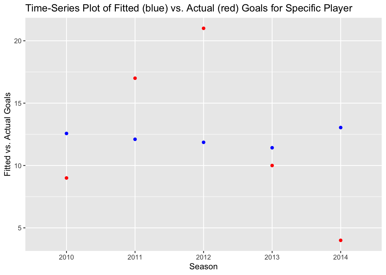
63.3.3.2 A random-effects model
Random-effects models assume that individual effects are uncorrelated with the other independent variables in the model. It assumes that the individual-specific effects are random and drawn from a common distribution.
These models consider both within-entity and between-entity variations. They allow us to analyse effects that do not change over time, providing a broader picture.
We’d use a random-effects model when we’rea interested in both the effects of time-varying and time-invariant variables and when the individual effects are assumed to be uncorrelated with the explanatory variables.
Random-effects model uses both within-entity and between-entity information, providing more efficient estimates under its assumptions than the fixed-effects model.
Let’s fit a random-effects model to the same player data:
# Fit a random effects model
re_model <- plm(goals ~ minutes_played + assists, data=players,
                model="random", index=c("player_id", "season"))
summary(re_model)
Oneway (individual) effect Random Effect Model
(Swamy-Arora's transformation)
Call:
plm(formula = goals ~ minutes_played + assists, data = players,
model = "random", index = c("player_id", "season"))
Balanced Panel: n = 10, T = 5, N = 50
Effects:
var std.dev share
idiosyncratic 66.308 8.143 1
individual 0.000 0.000 0
theta: 0
Residuals:
Min. 1st Qu. Median 3rd Qu. Max.
-14.1214 -7.1292 -1.2214 7.6701 14.7682
Coefficients:
Estimate Std. Error z-value Pr(>|z|)
(Intercept) 16.50730347 6.73338122 2.4516 0.01422 *
minutes_played -0.00071815 0.00223965 -0.3207 0.74847
assists 0.07574944 0.20430393 0.3708 0.71081
---
Signif. codes: 0 '***' 0.001 '**' 0.01 '*' 0.05 '.' 0.1 ' ' 1
Total Sum of Squares: 3355.8
Residual Sum of Squares: 3335.8
R-Squared: 0.0059505
Adj. R-Squared: -0.036349
Chisq: 0.281349 on 2 DF, p-value: 0.8687763.3.3.3 Check which model is more appropriate
The random effects model assumes that individual-specific effects are uncorrelated with the other predictors. This assumption should be tested using, for example, the Hausman test.
# Hausman test
phtest(fe_model, re_model)
    Hausman Test

data:  goals ~ minutes_played + assists
chisq = 15.14, df = 2, p-value = 0.0005157
alternative hypothesis: one model is inconsistent
This test helps us decide between the fixed and random effects models based on whether the unique errors (player-specific effects) are correlated with the regressors. In this case, with p <0.05, we can conclude that the fixed-effects model is appropriate as there is significant evidence that individual effects are correlated with explanatory variables.
63.3.4 How does this differ from classic time-series analysis?
Unlike time-series (which typically observes a single entity over time), panel data observes multiple entities. Panel data allows for controlling individual-specific traits that could influence the dependent variable. This data structure can uncover dynamics that are not observable in pure cross-sectional or time-series data.